
Sections
Proportional-integral-derivative (PID) controllers can handle most control problems if properly tuned. This article describes two basic methods of controller tuning.
Good process control relies on proper controller tuning. However, you must first understand the parts of the process to determine the necessary type of control. Part 1 of this article (June 2021, pp. 38–42) described some of the factors that may affect controller tuning and how to deal with them (1). Part 2 describes the basics of proportional-integral-derivative (PID) control and outlines two methods for tuning live systems without the need for tuning formulas or knowledge of equipment characteristics. Instead, the process itself provides the feedback information needed for proper control.
Basic PID control theory
A control system has three variables: the setpoint (SP), the process variable (PV), and the output (OP) (Figure 1). The PV is the parameter to be controlled (e.g., temperature, flowrate, etc.), the SP is the desired value for the PV, and the OP is the value sent from the controller to the control element.
▲Figure 1. This plot shows a typical proportional-integral-derivative (PID) control loop. The three main control variables are the setpoint (SP), process variable (PV), and output (OP).
For ease of description, we will use a flow that is controlled by a valve on a feed stream. When the value of the PV is not the same as the SP, the difference (PV – SP) is called the error. All of the controller actions are assumed to be based on this error value, although some controllers use the PV directly instead of the error for control of the derivative action, as discussed in later sections. Next, we review the standard PID controller and some of the factors that affect its operation.
Proportional (P). Proportional control responds to the error directly. This control method tries to stop the error from changing. As the error increases, the valve opening changes in direct proportion to the change. The tuning coefficient may be expressed as a proportional gain or a proportional band. If gain is used, increasing the coefficient will increase the response. Proportional band has just the opposite effect, where increasing the coefficient will decrease the response. Proportional gain is assumed in all of the examples used in this article.
Integral (I). Integral control, also referred to as reset control, responds to the total error. It tries to drive the PV back to the SP and drive the current error value to zero. This method works by constantly accumulating the error to calculate a total error value. The effect of the integral control is then proportional to this total. When the current error goes to zero, the total error stops changing. The integral tuning coefficient may be expressed as repeats/sec or sec/repeat, depending on how the PID equation is set up. Repeat is how often the controller comes back and looks at the error to adjust the OP.
When the integral tuning coefficient is expressed as repeats/sec, the response becomes stronger as the number increases. Alternatively, when the integral tuning coefficient is expressed as sec/repeat, the response becomes weaker as the number increases. The typical units are repeats/sec, but if you are unsure of the units for your system, make a small increase in the integral and see if the response gets stronger or weaker. Repeats/sec is assumed in all of the examples used in this article.
Reset windup is a problem that may arise with integral action. It occurs when the OP goes up to 100% or down to 0%. The integral (or reset) function continues to try and increase the OP to above 100% or below 0%. Mathematically, this occurs because the error continues to accumulate in the PID equation. This accumulation will delay the response when the error begins to fall and keep the OP from changing until the excess error that has accumulated is worked off. Reset windup is overcome automatically in most modern digital control programs. Once the OP reaches an upper or lower limit, the program stops the accumulation to prevent reset windup.
Derivative (D). Derivative control responds to the rate of change of the error. It tries to keep the slope of the error constant and does so by calculating the change in error vs. time (slope) for the recent time interval. The effect of the derivative control is then proportional to this slope. This provides a form of anticipatory control (rapid response) and can tighten the overall control. It can also cause unstable operation if not tuned properly. A sudden change in the PV in a system with derivative control could cause the OP to go to 100% or 0%, so it is not usually used (2). If you have a process where there are significant disturbances in the process inputs and the PV must be held within tight limits, derivative control may be needed.
If derivative control is active, a change in the SP will also be seen as a sudden infinite change in the slope of the error, which will significantly change the OP. Most control systems avoid this setpoint change effect by using changes in the PV rather than changes in the error for derivative control. The effect of derivative control is not part of the tuning discussed in this article.
Manual SP and OP changes. If a system is put into manual control, the automatic control is paused. During this time, the PV continues to track the actual value. Both the OP and SP may be changed manually by the operator while in this mode. When the system is put back on automatic control, it will use the current OP and SP values to restart its calculations.
Lag time. Lag time is the most significant problem that occurs in control systems. It is usually easy to tune a system that responds quickly to a change in the OP, but if the system has a long lag time, it must be tuned to react slowly enough so that cycling is not produced. Long lag time is usually overcome by using a control setting that is mostly proportional with a small amount of integral to bring the PV slowly back to the SP.
Basic control equations
The type of process control taught at the university level typically requires information on the valve type and size, lag times in the control OP and the process response, transfer functions for the process, etc. The methods described in this article consider all of these elements together as a “black box.” The total effect of all of these elements will be seen in the response of the control plots to a disturbance that is either provided by the process or created manually.
The standard form of the basic PID control equation is:

where OP is the output, K is the proportional gain constant, E is the error (PV – SP), I is the integral time constant, D is the derivative time constant, and t is time. The OP is proportional to E, the sum of E (ΣE), and the change in E over time (∆E/∆t). To use PID control in a simulation, it is often easier to use the velocity form of this equation. The velocity equation is a time derivative of the standard equation:

where OP1 and OP2 are the initial and current control outputs, respectively.
In Eq. 1, it is necessary to provide a value for the initial ΣE to produce the initial OP value. Then, you must keep up with the accumulated total error to generate the OP for each new time increment. The current OP is calculated from scratch every time and bears no relation to the previous OP. Equation 2 uses OP1 as a starting point and calculates the change caused by the change in error over the next time interval. Thus, the equation calculates an increment, and each new OP2 depends on OP1. This makes it much easier to describe and implement in a spreadsheet or computer program. The starting condition is then set simply by choosing a value for OP1.
Control systems can be direct-acting or reverse-acting. In a direct-acting system, an increase in the OP causes an increase in the PV. In a reverse-acting system, an increase in the OP causes a decrease in the PV. If we were applying chilled water to control a temperature, then increasing the valve opening (OP) would cause the temperature (PV) to decrease and it would be a reverse-acting system.
The type of controller action is an important factor in the control equations. In these equations, increasing the SP will cause the error to become more negative (i.e., if the SP goes above the PV, we would think of this as a negative error). For a direct-acting system, when the SP is above the PV, you want to increase the OP to increase the PV and drive it back up to the SP, which means the error term in Eq. 2 has to be positive. This is handled internally by the control system software. If you specify that you want a direct-acting system, the error will be calculated as (SP – PV). If you specify a reverse-acting system, the error will be calculated as (PV – SP).
Setpoint change tuning method
The first and most straightforward type of tuning is the setpoint change tuning method. This is a good tuning approach for systems that can be manipulated without significantly affecting the process, such as the feed rate to a product filter. It will be assumed that a rapid response type of control tuning is desired.
Before tuning, set up the SP/PV/OP plots and allow the system to stabilize, then increase the SP by a small amount (Figure 2). Observe the plots and see how they respond. In this example, the system overreacts. When the SP is raised from 900 gpm to 950 gpm, the valve (OP) opens too much and then cycles to find the solution. Either the proportional gain constant (K) or the integral time constant (I) is too large, or maybe both. The empirical way to tune in this situation is to eliminate the integral and then try again. The current values are K = 0.7 and I = 0.8. Write down these initial conditions and any changes that you make so that if any problems come up, you can always go back to the initial conditions. Also, be sure that you know how to put the system in manual control, if needed. If something gets out of control while tuning, put the OP under manual control and set it to the average value that it had when you started, then wait. After the PV returns to near the SP, set the control parameters back to where they were initially and then put the system back on automatic control until it stabilizes.
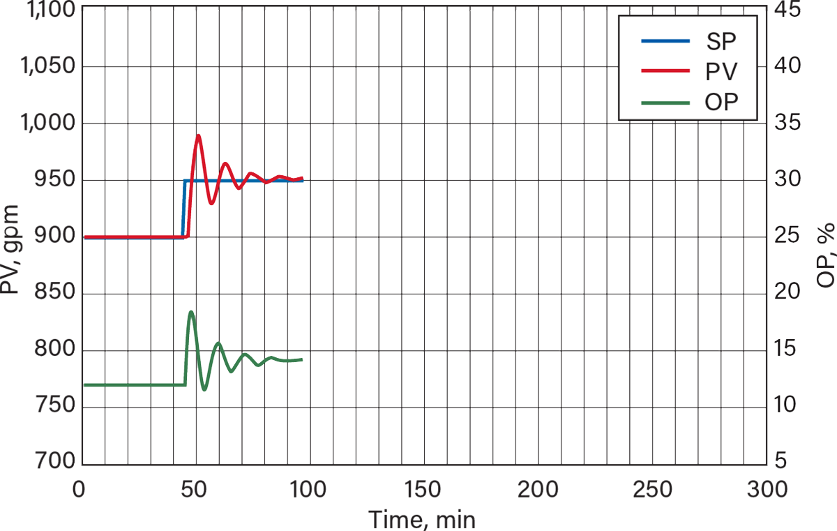
▲Figure 2. To begin the setpoint change tuning method, change the setpoint (SP) and see how the system reacts before any tuning. In this case, the system overreacts. Control parameters: proportional gain constant (K) = 0.7, integral time constant (I) = 0.8.
Step 1. Eliminate the integral control and see how the system responds. In this case, the integral is measured in repeats/sec, so we need to reduce the value to zero to eliminate the integral action. Figure 3 shows Step 1 of the SP change tuning method where you eliminate the integral effect and evaluate the effect of a change in SP with the current K value (i.e., K = 0.7, I = 0.0).
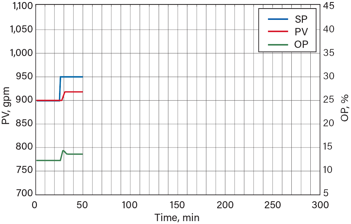
▲Figure 3. In Step 1 of the setpoint change tuning method, eliminate the integral (I) effect and evaluate the effect of a change in setpoint (SP) with the initial proportional gain constant (K) value. Control parameters: K = 0.7, I = 0.0.
The pure proportional control only brings the PV up to about 45% of the setpoint. The overshoot in the original plot was caused by having too much integral control. The proportional control provides the fastest and most stable response and is the least sensitive to a lag time in the system response, so it should be set to provide most of the control action.
Step 2. Increase the proportional control until the PV is roughly 70% of the SP. Typically, the proportional control should be set so that the PV reaches about 70% of the new SP. If the proportional K value is set too high, it will cause overshoot and cycling. Figure 4 shows the response when the K value is raised to 1.5. The proportional control now gets the PV up to 60% or 70% of the new SP.
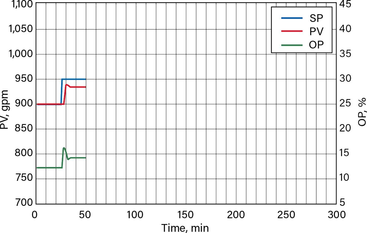
▲Figure 4. In Step 2 of the setpoint change tuning method, change the proportional (K) value to produce a response that is roughly 70% of the new SP. Control parameters: K = 1.5, I = 0.0.
Step 3. Add back in the integral control until the system responds as desired. Now that we have a good setting for K, more integral is added to complete the tuning. Figure 5 shows the response when the integral is increased to 0.3. The integral now pushes the PV up to barely past the SP and allows it to converge rapidly.
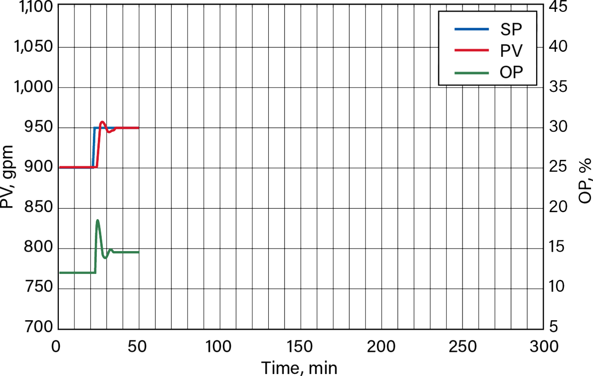
▲Figure 5. In Step 3 of the setpoint change tuning method, add the integral (I) control back until the system responds as desired. Control parameters: K = 1.5, I = 0.3.
In actual practice, these tests are performed sequentially with stepwise increases and decreases. The response from an increase may be slightly different than the response from a decrease, but it is seldom significant for this small range.
The full plot of the actual tuning session is shown in Figure 6. In the actual tuning session, the change in the SP was made from 900 gpm to 950 gpm, and the system stabilized at the new value. Then, I was set to zero, and the SP was decreased to 900 gpm again. The PV only moved about halfway toward the SP. At this point, I was changed to 0.5 to force the PV toward 900 gpm. Once the SP was met, the control settings were changed so that K = 1.5 and I = 0.0, then the SP was increased back to 950 gpm. This time, the PV went up by about 70%, which means the K value is now acceptable. The I value was then increased to 0.3 and the SP was lowered back to 900 gpm. The PV now came back to the SP rapidly and with only minor cycling. Once the tuning is done, it can be tested by moving the SP to higher and lower values and seeing how well the PV follows.
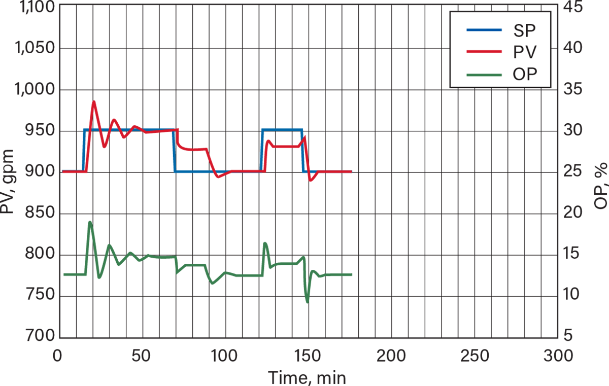
▲Figure 6. This PID plot shows what an actual setpoint change tuning session might look like.
The tuning process would be different if this had been a level control for a tank. In that case, only a loose control is needed, so the proportional parameter would be set to give a response of 20% to 30% of the SP change, and the integral would be set to some low value to move the level slowly back to the SP. The actual control parameters used would need to be strong enough to keep the tank level from getting too low (i.e., allowing the tank to empty) or too high (i.e., tank overflow or high-level alarm activation). This type of tuning is discussed later in the article.
Active process tuning method
In many cases, you will not be able to make significant changes to the SP because it will upset the process. In this case, an analysis of the patterns and interactions between the PV and OP may be used to tune the system, based on an understanding of the proportional and integral control behavior.
Before you begin the active tuning process, it is important to understand the objectives of the proportional and the integral controls. The proportional control merely increases or decreases the OP to stop the PV from changing. The proportional control does not try to bring the PV back to the SP; it only wants to slow it down and make it stop moving. You can think of this control as applying brakes on the system. The faster the PV is moving, the harder the system applies the brakes. If the PV is increasing, the system will try to slow down the rise. If the PV is decreasing, the system will try to slow down the fall. Once the signal is constant, the proportional control is satisfied.
The integral control, on the other hand, does want to force the PV back to the SP. The further away from the SP it is, the harder it pushes. As it gets closer to the SP, it pushes less and less. When it reaches the SP, it is satisfied and stops pushing entirely. The action of the control system is the result of the balance between the pushing of the integral and the braking of the proportional controls.
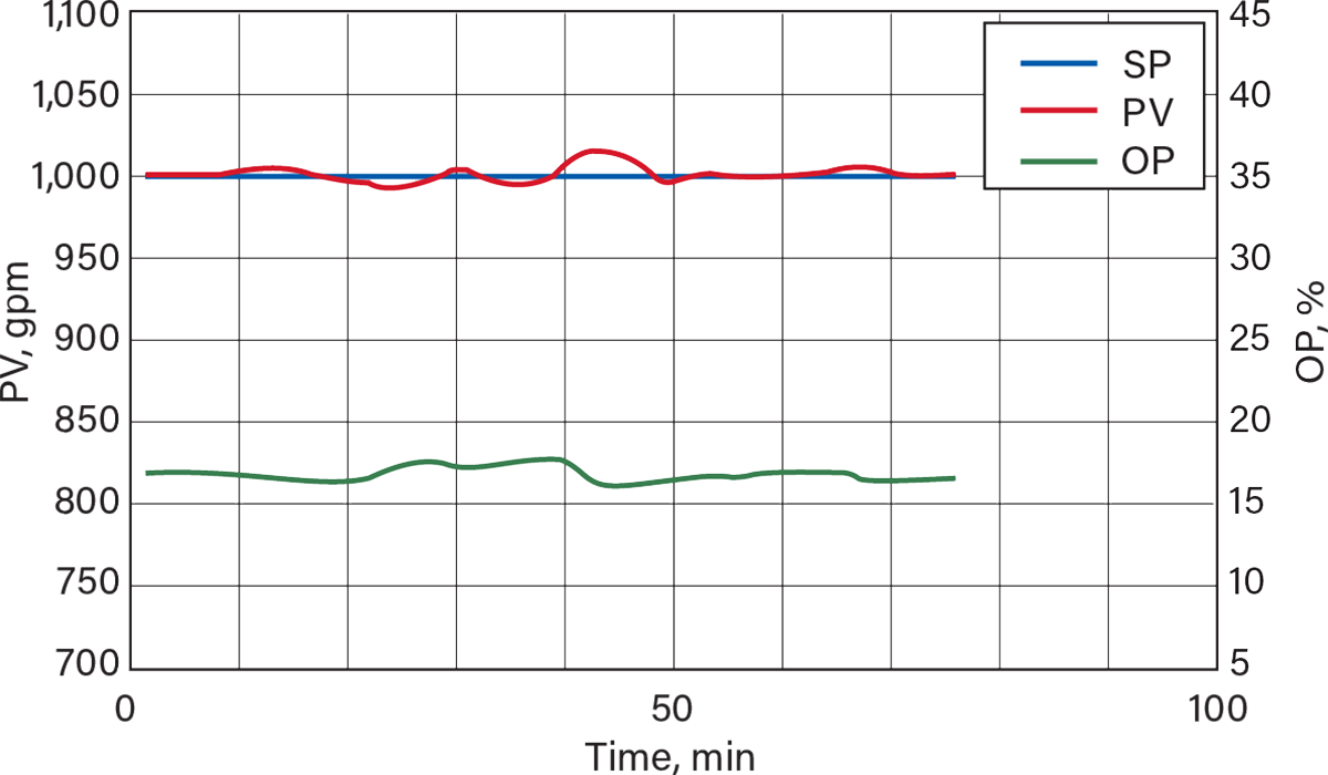
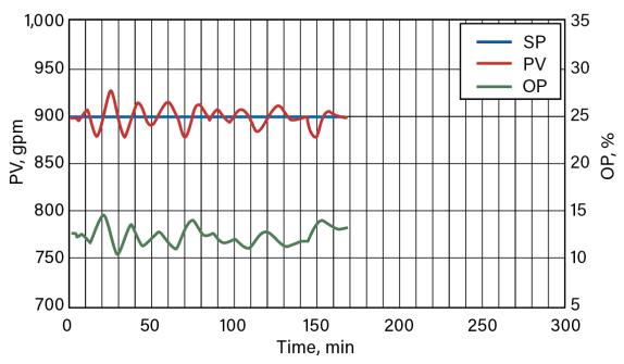
With this in mind, to tune an active system, first set up the control plot (Figure 7). An analysis of the wave patterns in Figure 7 shows that this is a direct-acting control system. In a direct-acting system, an increase in the OP causes an increase in the PV. The increase in the OP between 10 min and 20 min causes the flow (PV) to stop falling and go back up. In a reverse-acting system, an increase in the OP causes a decrease in the PV.

▲Figure 7. Analyze the control plot of the system before beginning the active process tuning method. This system is a direct-acting control system, which means an increase in the output (OP) causes an increase in the process variable (PV). Look for when the PV stops changing (e.g., 15 min, 24 min) to determine when the proportional control is satisfied. For example, at the top of the PV peak at 24 min, the OP curve shows a significant downward slope. This valve movement is from the integral part of the equation alone, so this controller has strong integral control. Control parameters: K = 0.5, I = 0.5.
This poorly tuned system can now be analyzed for improvement. When the PV of a system moves far past the SP and cycles, it is called an underdamped system. It could be overreacting because it is tuned too tightly or because the balance between the proportional and the integral controls is off.
Step 1. Determine which control type has a stronger effect on the system. Remember that the change in the proportional control is proportional to the change in error and the change in the integral control is proportional to the error itself (Eq. 2). When the proportional control is satisfied, it will stop applying the brakes, and all of the remaining control action is from the integral. In the same way, when the integral control is satisfied, it will stop pushing the PV toward the SP, and all of the remaining control action is from the proportional.
When is the proportional control satisfied? Proportional control is based on a change in the error, so it will be satisfied when the PV stops changing. This occurs when the slope of the PV plot equals zero. The slope equals zero at the top and bottom of the peaks in the PV curve. For example, look at the PV trough at 15 min in Figure 7; the OP curve has a significant upward slope at that point. At the top of the PV peak at 24 min, the OP curve shows a significant downward slope. This valve movement is from the integral part of the equation alone, so this controller has strong integral control.
When is the integral control satisfied? Integral control is based on the current error value, so it goes to zero when the error is zero. This occurs when the PV equals the SP. For example, look at the point where the PV curve crosses the SP curve at 11 min, 20 min, and 29 min in Figure 7. The slope of the PV curve is large, but the slope of the OP curve at those points is almost flat. This shows that the proportional part of the control is very weak, so most of the control is being done by the integral. (It is recommended to look at two or three points to evaluate the slope because the changing process values coming into the system will also affect the plots.)
Step 2. Slowly adjust the control constants until the system responds as desired. In this case, the integral appears to be too strong and is causing cycling. We could try applying more brakes (stronger proportional) or reducing the push (weaker integral). In this case, we will try to weaken the integral and see what happens. The current values are K = 0.5 and I = 0.5. The first adjustment will be to make I = 0.4 at 45 min (Figure 8). Once again, be sure to write down the initial conditions and any changes that you make.

▲Figure 8. In Step 2 of the active process tuning method, a small adjustment is made at 45 min to reduce the integral control. Control parameters: K = 0.5, I = 0.4 at 45 min. The PV peak at 60 min and the PV trough at 70 min (where the effect of proportional control is zero) show that the slope in OP generated by the integral control is lower, but still fairly strong.
The PV peaks at 60 min and 70 min (where the effect of proportional control is zero) show that the slope in OP generated by the integral control is lower than before we decreased I, but still fairly strong. The slope of the OP curve at the 73 min point where the effect of integral control is zero shows that the proportional control is still relatively weak. Next, we set I = 0.3 at 100 min in the second adjustment to reduce its effect even more (Figure 9).
▲Figure 9. The integral control is slightly decreased at 100 min to reduce its effect even more. Control parameters: K = 0.5, I = 0.3 at 100 min. The low points in the PV at 113 min and 149 min show that the slope caused by the integral is still significant, but getting smaller.
The PV low points at 113 min and 149 min show that the slope in OP caused by the integral control is still significant, but getting smaller. In addition, the deviation from the SP seems to be decreasing. At some points, the PV is holding at the SP instead of moving past it. Now, we will try making I = 0.2 at 170 min in a third adjustment (Figure 10).

▲Figure 10. In a third adjustment, the integral control is decreased even further. Control parameters: K = 0.5, I = 0.2 at 170 min. The PV returns rapidly to the SP and good control is now achieved.
At 175 min and 199 min, we can now see that the slope in OP is even smaller. In addition, you can see that when a deviation occurs, the control system brings it back to the SP and holds it there until the next deviation comes. For example, a bump begins at 170 min, and the PV returns to the SP at 182 min and remains there until the next bump. Another bump occurs at 194 min, and the PV is brought back to the SP by 207 min. The system is now slightly overdamped because the PV plot does not go much past the SP line. For this example system, the optimal I value is likely between 0.2 and 0.3. This tuning could also have been accomplished by increasing the K value and leaving the I value constant.
Once the system is tuned, if tighter control is needed, then both K and I should be increased together. If each is made more responsive but offset by the other, the whole system will react faster. However, the tighter the control, the more likely it is that a change in SP or a variation in the process will cause the control system to overreact and become unstable. Therefore, there is a limit to how much K and I can be increased. Figure 11 shows the control achieved when the parameters are doubled to K = 1.0 and I = 0.4 at 240 min. The response of the valve is faster, and the variations of the PV are smaller with these tighter control parameters. Once the tuning is complete, follow the plots for a few hours to verify the results. You should see that the variations are now much smaller under standard conditions.
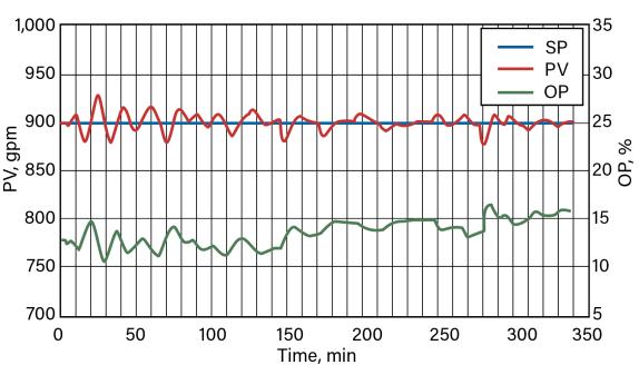
▲Figure 11. This plot shows the active process tuning method results where K and I are doubled, producing a tighter control. Control settings: K = 1.0, I = 0.4 at 240 min.
Figure 10 shows a system tuned for rapid response and Figure 11 shows a system tuned for tighter control. If this were a surge tank intended to even out the variations from the upstream process, it would need to be tuned more loosely. This is achieved by making it primarily a proportional control system with slight integral control to move the PV slowly back toward the SP.
As an example, we can look at a surge tank with two takeoff streams. One stream takes small batches out for purification and recycle and the other uses level control to provide a feed to the downstream process (Figure 12). The level controller has settings of K = 0.1 and I = 0.01. As the tank slowly empties, the level control valve closes, but does not move rapidly enough to drive the level back up to the SP. Batches of liquid are removed until a new batch of feed is provided, and the level goes back up. The discharge of this tank (represented by the %OP), which feeds another part of the process, is much more stable than if the system were tightly controlled to maintain the level.

▲Figure 12. In this example, loose control is desired in a surge tank with two takeoff streams. Loose control is achieved by making it primarily a proportional control system with slight integral control to move it slowly back toward the setpoint. Control settings: K = 0.1, I = 0.01.
Cascade control
Cascade control is another important type of process control, and perhaps one of the most difficult to tune. This type of control is necessary when the parameter used to provide the control varies with time. A good example is the steam flow to a distillation column reboiler. If the steam pressure is constant, a temperature control loop can adjust a valve on the steam line directly and it will work fine. However, the pressure in a steam header will often vary based on the demand from several processes that are using it at the same time. There can even be pressure variations from the steam boiler operation itself. In this case, a separate control must be used to adjust the steam flowrate. A temperature controller controls the SP for this flowrate, i.e., the OP from the temperature controller is sent to the steam flow controller as a SP. This means that the temperature controller is the primary controller and the steam flow controller is the secondary controller. The steam flow controller adjusts the valve to produce the flow requested by the temperature controller. This will compensate for any variations in the pressure of the steam.
For these control systems, the secondary controller should be tuned for tight control and the primary controller should be tuned for loose control to avoid cycling. The goal of the secondary controller is to move rapidly to the target while the primary controller moves that target slowly. If the target is moved too fast, the secondary controller will not be able to keep up. By the time it reaches the target, the PV has already gone too far and the primary controller is moving the target back in the other direction. This leads to cycling as the system constantly searches for a solution.
Take the following steps to tune cascade control systems:
- Set up two PID plots as shown previously — one for the primary controller and one for the secondary controller. Monitor the SP that the primary controller provides to the secondary controller and find the average value. Also, find the average value for the OP of the secondary controller. This is the actual control element for the system. If a problem occurs during tuning, put the secondary controller on manual and set its OP to this value to bring the system back under control.
- Record the control variable values (K and I) for both loops for future reference.
- If the system does not have much variation, put the primary controller on manual and set its OP (the SP for the secondary controller) at its average value. This should keep the system operating in its normal range. If the system does have significant variation, then use the active process tuning method to try and tune the secondary controller based on how it responds to the SP from the primary controller. Make small tuning adjustments in this loop so that the secondary controller more closely follows the moving SP.
- Once the primary controller has been set to manual, tune the secondary controller as described above using the setpoint change tuning method. Make small changes in the OP of the primary controller and watch the results. By making a positive change followed by a negative change, you can make them average out and not disturb the process too much.
- Once the secondary controller is tuned and tracking well, put the whole system back in automatic mode and see how it performs.
- Now proceed to tune the primary controller using the active controller tuning method. In some cases, the system may now be so stable that this method cannot be used. In that case, use the SP change method to test the primary controller loop and see if it needs further tuning. Remember that when tuning this loop, you should tune it to react slowly and allow time for the secondary controller to catch up. Since cascade control introduces a longer lag time, use more proportional and less integral control in the primary controller to improve stability.
- Monitor the system for several hours to ensure that changes in the process conditions do not cause stability problems.
In closing
Simple PID controllers can handle most control problems if properly tuned. First, determine what kind of control you need: rapid, tight, loose, or cascade. Then, use the methods described in this article to achieve the desired control. The active process tuning method is particularly suitable for sensitive systems, while the setpoint change tuning method is more suitable for rugged systems.
Nomenclature
| D | = derivative time constant |
| E | = error |
| I | = integral time constant |
| K | = proportional gain constant |
| OP | = output |
| OP 1 | = initial output |
| OP 2 | = current output |
| t | = time, min |
Literature Cited
- Reed, H., “Empirical Process Control: Part 1,” Chemical Engineering Progress, 117 (6), pp. 38–42 (June 2021).
- Rohani, S., “Coulson and Richardson’s Chemical Engineering: Volume 3B: Process Control,” Fourth Ed., Butterworth-Heinemann, Oxford, U.K. (2017).

Copyright Permissions
Would you like to reuse content from CEP Magazine? It’s easy to request permission to reuse content. Simply click here to connect instantly to licensing services, where you can choose from a list of options regarding how you would like to reuse the desired content and complete the transaction.